JBCS

INTRODUCTION

The Ehrenfest Urn Model (EUM), or as it is also named, the Stochastic Monte Carlo Method,^1-4 was developed to statistically prove Boltzmann's H Theorem, which describes the irreversible route to thermodynamic equilibrium.⁵ The standard Ehrenfest Urn Model consists of two urns filled with numbered balls. The process is characterized by the extraction and the reallocation of numbered balls between the urns using random numbers. That process proceeds until the thermodynamic equilibrium is reached.³ The chemical kinetic equations⁶ can also be solved by using the EUM in order to describe the thermodynamic equilibrium and steady states.

The Practical Stochastic Model (PSM) can be compared with the Stochastic Simulation Algorithm (SSA) as developed by Gillespie⁷ and to the lattice-gas automata techniques.^8,9 However, the PSM was developed independent of those methods and is significantly easier.

The development of the PSM was based on the earlier works for simple first and second order reactions^4,10 and was then expanded to non-linear reactions. The non-linear systems addressed in this work are formed by the different classes of coupled reactions, where the chemical species are present in two or more different (kinetic rate) equations. That dependence of the kinetic behavior of the chemical species in different kinetic rate equations is responsible for creating polynomial terms in a different form of linear in the rate law. The concept of non-linearity in chemical systems comes from that fact. A particular class of reaction, which has capital importance, is the autocatalytic process. These reactions are responsible for the concentration of oscillation of the intermediary chemical species. For example, the reaction X+Y→2X is a bimolecular reaction, since two substances participate in this reaction step. This reaction can also be nominated as a unimolecular autocatalytic reaction, since the catalytic substance only appears once in the reactant side. The reaction 2X+Y→3X is a trimolecular reaction, or a bimolecular autocatalytic one, based upon similar discussions as above.¹¹ A classical non-linear chemical reaction is the Belousov-Zhabotinsky reaction. It is an important example of dynamic chemical systems, composed of more than one chemical step, and among those steps, autocatalytic reactions.¹¹

Some definitions concerning the theory employed in this study are to be considered as follows: 1) Stochastic - a Numerical Method that considers a time evolution of a discrete chemically reacting system;⁷ 2) Monte Carlo Method - a Mathematical Tool for integrating an ODE based on random sampling;¹ 3) Deterministic - a Numerical Method that considers the time evolution of a continuous chemically reacting system;⁷ 4) Non-Linear ODE - A set of coupling Ordinary Differential Equations with polynomial degree terms higher than one (linear);¹² 5) Steady State - a Solution of ODE where the value of a dependent variable (concentration) does not change over time;¹² 6) Stability of ODE - a Linear Behavior (stable or unstable) around the steady state;¹² 7) Trace (tr) of Stability Matrix - the Sum of Eigenvalues of a Linearized ODE: tr<0 (stable); tr>0 (unstable).¹²

The initial Monte Carlo studies,^4,10 mainly for first order reactions, have been considered in several other works:^13-16 a) Luminescence and Kinetics of Excited States Decay;¹³ b) Transfer Mechanism of Electronic Excitation Energy: Perrin Model for Static Suppression of Luminescence;¹⁴ c) Study of Homogeneous Chemical Reactions;¹⁵ d) Simulation of the Suppression Mechanism of Luminescence: Kinetic Model of Stern-Volmer.¹⁶

The PSM method can accurately describe the linear and non-linear chemical kinetic reactions, where the fluctuations are naturally obtained, simulating the finiteness of the systems. This method is consistent, robust, simple, practical, and independent of a deterministic Ordinary Differential Equation (ODE). The PSM is a simple model of a "particle" exchange between containers, where the state of the system is defined in terms of the container occupancy.⁴ The system's evolution is driven by state dependent transition probabilities, which depend on the occupancy. The PSM could be considered as a simple and practical reformulation of the SSA. This equivalence can be defined by just introducing containers as chemical species and the transition probabilities as reaction propensities. The main advantages of the PSM, which give absolute values, are: simplicity, efficiency, and intuitiveness.

This method has already been used for many years in the classroom to simulate the kinetic behavior of first and second order reactions. To introduce the method, a vector with only 10 positions can be used with a manual random selection. 10 is a good number to perform a manual selection, as it is small enough to manually realize first order kinetics in approximately 15 minutes (with second order reactions, the time increases as N²) and is large enough to avoid strong fluctuations that could obliterate the visualization of the kinetic behavior. It is necessary to use a computer to carry out simulations for a large N.

This method is a very easy and efficient statistical integration tool and avoids the use of more advanced mathematical techniques, but still allows for accurate descriptions of the various chemical aspects related to reactions, including the relaxation time (the necessary time for a reaction to reach equilibrium); thermodynamic equilibrium and fluctuations; and a description of the steady states. This method is efficient for teaching chemical kinetics and becomes a very powerful tool in a simple way for simulating chemical reactions.

METHODOLOGY

The PSM was built step-by-step with simple (first and second-order) reactions, and it was completed considering non-linear reactions as do the Lotka¹⁷ and the Brusselator¹² systems. The parameters and variables of the stochastic method were initially adjusted to the deterministic method (ODE) in order to establish the main rules of this particular stochastic one. These rules are: a) N-scale - parameters, variables, and time were scaled by N (the total number of positions); b) Dilution (d) - compartment filling or vector occupation, which represents the "particle concentrations"; c) m-rate - the rate of the reaction enhancement, which indicates how many times one reaction must be repeated in order to obtain the true concentration of variables from a normalized vector occupation. The N-scale was established with first and second order reactions; d and m were revealed considering the Lotka model system.

The PSM is based on Monte Carlo steps and could be compared to the Stochastic Simulation Algorithm (SSA) as developed by Gillespie⁷ (see Supplementary Material (SM) - Section A.1: Figure 1S and Figure 2 for reference).⁷ Zhdanov⁸ also considers the Monte Carlo method in order to solve the Brusselator system, which is shown in SM (Section A.2).

The PSM approach was developed for comparing its solution to the deterministic methodology. This stochastic simulation assumes that the compartments can have any occupation from 0 to N, which represents the concentration variables. The dilution variable (d) is defined as the vector occupation divided by the total number of positions (N). d is numerically equal to a p probability to find a particle in the vector.

The necessary steps to simulate a typical reaction are (as in the explicit example that is given in Supplementary Material (SM) - Section A.3):⁴

I Randomly select a number from 1 to N; if the position at the same selected number, in a specific compartment, is occupied (by a "particle"), then its "particle" is withdrawn from this place and is relocated in another compartment at the same number position with a q probability. This process chemically represents the conversion, e.g., of A to B. This probability of q is connected to Arrhenius' equation, which is a function of the activation energy, orientation, cross section, and molecular velocity, for real systems. The p probability of finding the "particle" in the compartment is numerically equal to dilution, which is connected to the density of the particle (i.e., concentration).

II Randomly select other number from 1 to N and a similar procedure as above is considered for other "reagents".

III After running these above steps, the all-step-procedure is restarted and repeated until it reaches an equilibrium or a steady state.⁴

IV When the position corresponding to a randomly selected number is empty, it means that no reactions are occurring, but the time flow continues, i.e., the number corresponding to the Monte Carlo step is also computed.

In order to simplify the discussions, it is assumed that q=1, however, the values of q for 0<q< 1 can also be considered, for example, as in the Lotka model¹⁷ (see below and in the SM), and was solved for different values of q.

In the PSM approach, the step size time is effectively proportional to 1/N. This procedure would be equivalent to the Euler method, with the step size converging to zero for increasing N. The PSM completely describes the chemical kinetic reactions and it can be extended using non-null diffusion constants and dimensions higher than one. More details are discussed in following sections.

RESULTS AND DISCUSSION

In the first step, it was necessary to establish connections between the stochastic method and the deterministic method. For that, several kinds of chemical reactions were used, in order to obtain the main stochastic rules. Those rules are simple and intuitive and contribute to an understanding of the method and its generalizations. Finally, the developed stochastic method is very accurate and can potentially describe any kind of chemical kinetic reaction. The main steps of those connections are given below:

Stochastic and deterministic connections: time flow

The stochastic and deterministic time flow connections were obtained from several simulations (see SM - Section B). The flow of time obtained from the deterministic solution is numerically equivalent to the number corresponding to the Monte Carlo step divided by N, where N is the size of the system, or the size of the compartments. The compartments could not be fully occupied.

Each step of the first order reaction occurs with a probability (p) equal to dilution (d). Equivalently, the probability of p for each second order reaction step is equivalent to the product of dilution. The stochastic simulations describe this statistically.

The first and second-order reactions of the stochastic approach can be described by (scaled) relative values of the concentrations (parameters and variables). However, a set of coupled non-linear reactions should be described by absolute values. For example, the stability matrix trace (tr)¹² of the non-linear system depends on the absolute values such as, e.g., tr = q₂B-q₄-q₃ (q₁A/q₄)² or tr = B - 1 -A² (with unitary probabilities) for the Brusselator system, where A and B are the concentration parameters (SM - Section A.2). For example, if one can correctly describe the concentration evolution in time for the Brusselator system with tr>1, it is necessary to require that B>1.

Stochastic and deterministic connections: absolute concentrations

In order to develop a concise stochastic theory, it is necessary to understand the relationship between the stochastic and deterministic methods for the absolute values of the concentrations (parameters and variables). It is easier to start the analysis firstly by considering the absolute values of concentration parameters (e.g., A) bigger than unity with concentration variables less than unity. The parameters are ever constants for deterministic and stochastic methods. They can be understood as reagents or products, which are consumed or produced, but are kept as constants, on average, for a stochastic method.

If [A] < 1 is the numerical value of [A], obtained from the above stochastic method, it is similar to that of a deterministic one. However, if [A] > 1, it is necessary to use a "reservoir" for the A parameter, since it is not possible to have N_A>N. In other words, it is necessary to increase the probability, by adding more random selection steps to the reaction, especially where the A parameter appears, in order to overcome that limitation.

That step must be m-repeated in order to increase the probability (by addition), in order to obtain the true concentration. The factor m or the rate of reaction enhancement can be interpreted as increasing the collision factor by the "density" of the concentration. The concentration [A] can then be defined as [A] = mN_A/N.

Several combinations were performed to show the correctness of the relation [A] = mN_A/N; the main difference appears in the fluctuation amplitude; since this depends on N^{1/2 18} (see SM - Section C), the relation of [A] = mN_A/N is trivially obtained. That relation means that the time flow decreases m-times, while the velocity and the concentration become m-times larger.

Similarly, one can also study the absolute values of the dependent variables (e.g., X) that are greater than unity. In this case, the m-factor is now a variable, i.e., it changes with the progress of the reaction. In order to describe that, it is necessary to implement an "adjustable reservoir" (or accumulator), where the excess of the compartment, e.g., X, is added to it. That is, if [X] (> 1), then formally N_X = [X] N, and the excess is given by Ex = N_X - N = ([X] - 1) N, where N is the maximum number of occupations of the X compartment, as defined above. A relative excess can be defined as e = Ex/N.

The real number r = 1+ e = (N + Ex)/N = N_X/N = [X] is taken into account when [X] > 1. A natural number m can be defined by the application of a truncation operation over r, i.e., m = trunk (r). The usual procedure does not change if r< 1, i.e., just choosing the random number (m=1) once is enough. However, if m= trunk (r) > 2, it is necessary to add (m - 1) random choices.

If [X] > 1, the difference between r and m, i.e., the relative excess e = r - m, must be added to an "accumulator" (acc) for each random chosen step. It is necessary to accumulate that difference, since it is not possible to make a fractional number of random selections. When the accumulator exceeds the unit, additional random choices are carried out in the same step, and the accumulator suffers a reduction. For example, the random choice must be carried out when r = [X] > 1 and the excess (e = r - m) is added to the accumulator, acc' = acc + e. At the next step, a new r = [X] is obtained, and a new excess e' is added to the accumulator, i.e., acc'' = acc' + e'. After k-random selections, the accumulator could exceed the unit (acc> 1) and the number of random choices could usually increase by one unit, i.e., m=1 changes to m=2. In that case, the accumulator must decrease itself by one unit. This procedure should be done when [X] >1.

The general PSM scheme is shown in SM - Section A.1. The complete flowchart for the A+X→Y reaction (as discussed in SM - Section C) is shown below:

Non-linear reactions

The Lotka¹⁷ and Brusselator¹² non-linear chemical reaction systems were studied with the stochastic method, as is described below:

Lotka system

The Lotka system is described by three reactants: one parameter (A) with a constant concentration and two variables (X and Y) as chemical intermediaries: X+Y→2Y; A+X→2X; Y→P with kinetic constants q₁, q₂, and q₃, respectively. These reactions are described by the following ODE's: d[X]/dt=q₂AX-q₁XY and d[Y]/dt=q₁ XY-q₃Y. This system implicitly considers a constant flux, since A and P are substances with a constant concentration.

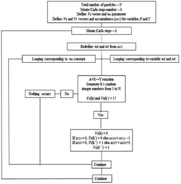Figure 1. Flowchart of the stochastic method for an A+X→Y reaction

The deterministic solutions X(t) and Y(t) of the Lotka system for q₁ = 0.5, q₂ = 0.6, and q₃ = 0.7, A=4, X₀=1, and Y₀=1.5, as obtained by the Runge-Kutta method, are shown in Figure 2, where X₀ and Y₀ are the initial conditions. The stochastic solutions, considering the procedures of Section 3.1 and Section 3.2, are also shown in Figure 2 for A=10000/10000=1 with m_A=4 (A=4), X₀=10000/10000=1, and Y₀=10000/10000=1 with acc_Y = 5000/10000=0.5 (Y₀=1.5) and with the same q's as above.

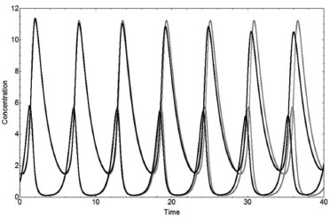Figure 2. Concentrations X(t) and Y(t) as a function of time for the Lotka system using q₁ = 0.5, q₂ = 0.6, and q₃ = 0.7, from a deterministic method (gray lines) with A=4, X₀=1, and Y₀=1.5, and from the stochastic solution (black lines), with N_A=10000 (m_A=4), N_X=10000, N_Y=15000, and N=10000

The occurrence of a limit cycle in the space of configuration (X vs. Y) is shown in Figure 3 for the two methods:

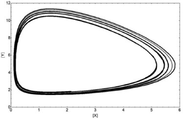Figure 3. Limit Cycle for the Lotka system obtained from both methods. Similar comments are as in Figure 2

This simple stochastic method describes the Lotka system very well when compared to a deterministic one. The absolute values of the parameters and variables and the oscillations are correctly described. The "dissipative" aspect as shown in the limit cycle is due to the finiteness of the system. That aspect could be interpreted mathematically as a numerical error for a deterministic map approximation.¹⁹ A Fortran code program for Lotka system is shown in SM - Section D.

Brusselator system

Other non-linear coupled chemical reactions were studied and were contemplated by using the Brusselator system, which has a trimolecular reaction (or bimolecular autocatalysis). Its chemical reactions are: A→X; B+X→Y+D; 2X+Y→3X; and X→E, with unitary kinetic constants, i.e., q₁ = q₂ = q₃= q₄ = 1. This system is described by four reactants: two parameters (A and B) with a constant concentration and two variables (X and Y) as chemical intermediaries. These chemical equations are described by the following ODEs: d[X]/dt= A-(B+1) X+X²Y and d[Y]/dt=BX-X²Y. This system has important differences on stability behavior when in comparison to the Lotka one.¹²

The deterministic solutions X(t) and Y(t) of the Brusselator system for A=0.5, B=1.4, X₀=1, Y₀=1, and tr=0.15 (the trace of stability matrix)¹², are shown in Figure 4. The stochastic X(t) and Y(t) ones for A=5000/10000=0.5, B=7000/10000=0.7 with m_B=2, i.e., B=1.4 and X₀=Y₀=10000/10000=1 are also shown in Figure 4.

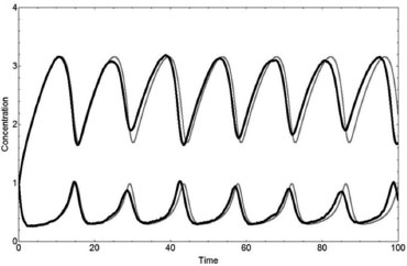Figure 4. Concentrations X(t) and Y(t) as a function of time for the Brusselator system using q₁ = q₂ = q₃= q₄= 1 from the deterministic method (gray lines) with A=0.5, B=1.4, X₀=1, and Y₀=1 - and from the stochastic one (black lines) with N_A=5000, N_B=7000 (mB=2), N_X=10000, N_Y=10000, and N=10000

The occurrence of a limit cycle in the space of configuration (X vs. Y) is shown in Figure 5 for both methods:

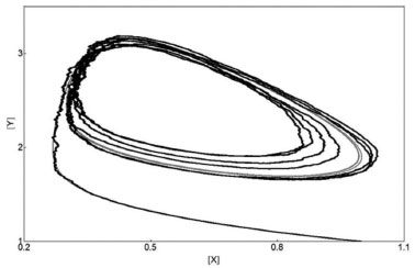Figure 5. Limit Cycle for the Brusselator system from both methods. Similar comments as in Figure 4

The PSM describes the Brusselator system very well when compared to the deterministic method. The absolute values of the parameters and variables and the oscillations are correctly described by the Lotka and Brusselator systems. However, the response of the stochastic method is slow when in comparison to the deterministic one, if the derivatives dX/dt and dY/dt have large values. For example, the sharp oscillations are not reproduced by the Brusselator stochastic model with A=5000/10000=0.5, B=8000/10000=0.8 with m_B=3, i.e., B=2.4 and X₀=Y₀=10000/10000=1 for the stochastic method when in comparison to A=0.5, B=2.4, X₀=1, Y₀=1, and tr=1.15 for the deterministic one. These deterministic and stochastic solutions X(t) and Y(t) of the Brusselator system are shown in Figure 6.

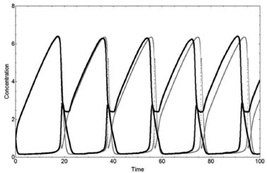Figure 6. Concentrations X(t) and Y(t) as a function of time for the Brusselator system using q₁ = q₂ = q₃= q₄= 1 from the deterministic method (gray lines) with A=0.5, B=2.4, X₀=1, and Y₀=1 - and from the stochastic one (black lines), with N_A=5000, N_B=8000 (m_B=3), N_X=10000, N_Y=10000, and N=10000

A zoom of the concentrations X(t) and Y(t) for both methods and their respective deterministic derivatives are shown in Figure 7. The slow response to describe the maximum of the X variable and a minimum of the Y one, from the above example, is shown in detail in Figure 7. The slow response does not change by increasing the number of particles N. However, an irregular sharpness appears with a decrement of N. Similar features can be seen in Zhdanov's work for the Brusselator system.⁸

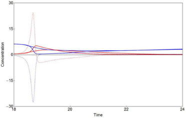Figure 7. [X] deterministic and stochastic (red solid lines) and d[X]/dt deterministic (red dashed line); [Y] deterministic and stochastic (blue solid lines) and d[Y]/dt deterministic (dashed blue line) for the Brusselator system. Similar comments as in Figure 6

The stochastic method can show a "slow" response to adjust to the sudden changes of variables, perhaps due to the discreteness of m. Another tentative was considered in order to minimize the discreteness of the variables of m. For example, at each step, the non-integer part of the relative excess e = r - m< 1 was interpreted as an additional probability (s_a). Such a consideration of s_a was used in another additional random selection, avoiding the use of an accumulator. The responses of both exploratory tests are virtually identical.

Generic chemical reactions can be described by different techniques such as the ODE approach (an infinitesimal description), or by a stochastic simulation (a discreteness description), which are the first principle procedures using a different nature. One can consider that the "slow" response of the stochastic method (see above), in comparison to the deterministic one, could be a best answer of the real chemical reactions, since the ODE approach is an infinitesimal description of chemical reactions, which essentially have a discrete nature.

These two non-linear systems are described correctly by the Practical Stochastic Method, which is simple, robust, auto-sufficient, and independent of a deterministic procedure. This stochastic model can achieve absolute values, which is very important, in order to describe non-linear reactions.

CONCLUSIONS

The PSM is an improvement over the simple Ehrenfest Urn model, which is based on the random selection of compartment positions, in order to describe the path of equilibrium in simple chemical reactions.⁴ This improved method adds some precise rules, with a simple implementation, to correctly describe the steady state route of non-linear chemical reactions.

The connection between the stochastic and deterministic methods was established in order to achieve a consistent stochastic one. For that, it was necessary to define two main concepts: a) the filling of the compartment, or by dilution; b) the rate of the reaction enhancement.

This simple stochastic method is an alternative to describe finite chemical kinetic reaction systems, where fluctuations are naturally obtained. This stochastic method is robust and is a consistent approach in possible applications for linear and non-linear chemical systems. The "Practical Stochastic Model for Chemical Kinetics" can manage absolute values, which is very important, when describing non-linear reactions.

ACKNOWLEDGMENTS

The financial support given by the Sao Paulo Research Foundation (FAPESP, Fundaçao de Amparo a Pesquisa do Estado de Sao Paulo) Grant 2010/11385-2 and by the CNPq (Brazilian Science Funding Agencies) is fully acknowledged with special thanks.

REFERENCES

1. Metropolis, N.; Rosenbluth, A. W.; Rosenbluth, M. N.; Teller, A. H.; Teller, E.; J. Chem. Phys. 1953, 21, 1087. DOI: http://dx.doi.org/10.1063/1.1699114

2. Metropolis, N.; Los Alamos Sci. 1987, 15, 125.

3. Prestipino, S.; Physica A 2004, 340, 373. DOI: http://dx.doi.org/10.1016/j.physa.2004.04.029

4. Lopez-Castillo, A.; Souza-Filho, J. C.; Quim. Nova 2007, 30, 1759. DOI: http://dx.doi.org/10.1590/S0100-40422007000700045

5. Ehrenfest, P.; Ehrenfest, T.; Phys. Z. 1907, 8, 311.

6. Moore, W. J.; Physical-Chemistry, 4^th ed.; Longmans Green & Co. Ltd.: Harlow, 1963, 804p.

7. Gillespie, D. T.; J. Chem. Phys. 1977, 81, 2340. DOI: http://dx.doi.org/10.1021/j100540a008

8. Zhdanov, V. P.; Phys. Chem. Chem. Phys. 2001, 3, 1432. DOI: http://dx.doi.org/10.1039/b100192m

9. Kawczynski, A. L.; Gorecki, J.; Nowakowski, B.; J. Phys. Chem. A 1998, 102, 7113. DOI: http://dx.doi.org/10.1021/jp9807118

10. Braga, J. P.; Físico-Química: Aspectos Moleculares e Fenomenológicos, Ed. UFV: Viçosa, 2002, cap. 1.

11. Epstein, I. R.; Nature 1995, 374, 321. DOI: http://dx.doi.org/10.1038/374321a0 PMID: 7885470

12. Prigogine, I.; Nicolis, G.; Self-Organization in Non-Equilibrium Systems: From Dissipative Structures to Order through Fluctuations, 1ª ed., John Wiley & Sons: New York, 1977, chap. 7.

13. Winnischofer, H.; de Araújo, M. P.; Dias Júnior, L. C.; Novo, J. B. M.; Quim. Nova 2010, 33, 225. DOI: http://dx.doi.org/10.1590/S0100-40422010000100039

14. Novo, J. B. M.; Dias Júnior, L. C.; Quim. Nova 2011, 34, 707. DOI: http://dx.doi.org/10.1590/S0100-40422011000400027

15. Farias, R. R.; Cardoso, L. A. M.; Oliveira-Neto, N. M.; Nascimento Junior, B. B.; Quim. Nova, 2013, 36, 729. DOI: http://dx.doi.org/10.1590/S0100-40422013000500020

16. Dias Júnior, L. C.; Novo, J. B. M.; Quim. Nova 2014, 37, 361. DOI: http://dx.doi.org/10.1590/S0100-40422014000100027

17. Lotka, A. J.; J. Am. Chem. Soc. 1920, 42, 1595. DOI: http://dx.doi.org/10.1021/ja01453a010

18. Delbrück, M.; J. Chem. Phys. 1940, 8, 120. DOI: http://dx.doi.org/10.1063/1.1750549

19. Lima, M. R.; Claro, F.; Ribeiro, W.; Xavier, S.; Lopez-Castillo, A.; Int. J. Nonlinear Sci. Numer. Simul. 2013, 14, 77.