JBCS

INTRODUCTION

The problem of teaching chemical kinetics has been discussed in many works on teaching approaches.¹ However, one must not forget about the role of the experiment.² It is only the laboratory practice that really allows to understand the complex problems of kinetics associated with the choice and optimisation of the conditions of an experiment, the interpretation of results as well as the perception of potential and actual sources of errors at the stage of experiment and at the stage of data analysis. In the following paragraphs, we will describe those aspects by taking as an example the hydrolysis reactions defined by a simple mathematical model (see equation 1).

As part of their laboratory class on chemical kinetics, students analyse, inter alia, reactions consistent with first and pseudo-first order mechanisms, e.g. the kinetics of acidic and base hydrolysis of esters as well as the inversion of sucrose (hydrolysis). This last example and the progression curves analysis were described, for instance, in the work of M. J. J. Holt and A. C. Norris.³ Those reactions are relatively slow and thus can be scrutinised using classical methods. For such cases, the following equation (1) is used to describe the progression curve of a reaction:⁴

or, after linearisation:

where: C₀ - concentration of substrate at the start of measurement (t = 0); C - instantaneous concentration of substrate in time t.

Given that many measured physicochemical parameters of a reacting system are directly proportional to the concentration, they can be directly used in the equation (2), without the need to calculate instantaneous values of concentration (e.g. using a calibration curve).^5,6 This makes it possible to avoid the additional source of errors, the observed rate constant (the estimated parameter in this equation) being expressed in the correct unit (1/s). However, some of the measured physicochemical parameters are additive and do not change in the range (Y₀, 0) if the loss of substrate is being examined or (0, Y_max) - if the increase of product is tracked during the reaction time. The said parameters change in the range (Y₀, Y_∞) respectively. From this it follows that once the proportionality of changes of the measured parameter with regard to the concentration has been taken into account, the equations (1,2) will each respectively take the following forms:

or a more commonly used form of:

where: Y - measured parameter of a reacting system, proportional to the concentration; Y_∞ - limit value (asymptote) of the measured parameter of a reacting system.

While the measurement of value of Y does not pose a problem - it is simply the instantaneous value of the parameter measured in time t, the determination of value of Y_∞ is not so straightforward. Textbooks and publications that consider the above-shown type of reaction usually provide methods of determining Y_∞ experimentally.^5,7 Nevertheless, as our experience shows, this is associated with a risk of multiple errors that significantly affect the end result obtained. It is not always the case that inexperienced students notice this. Yet another difficulty is that in order to determine Y_∞ experimentally, some reactions would have to be tracked for several days, which is hard to achieve in a laboratory class. In the literature, one finds both a number of methods for determining Y_∞ mathematically as well as proposed methods for calculating the rate constant without the need to calculate or determine Y_∞ and Y₀.^8,9 Given that computer software is widely available (spreadsheets), some of those historical methods are rather outdated, for instance, those based on graphical determination of the slope of tangents to the progression curves.⁸ However, it should be noted that this approach does have some didactic value. Other proposed solutions seem to be too difficult for undergraduate students.¹⁰

Below, on the basis of selected progression curves, we will prove that, given the experiment has been conducted carefully, the needed value of Y_∞ can be found iteratively, thus obtaining better accuracy at considerably reduced experiment duration. In addition, sometimes it seems to be the only reliable method. For this purpose, the equation (3) may be used, after it has been rearranged to arrive at the following:

The use of a nonlinear fitting method (e.g. Levenberg-Marquard algorithm) makes the experimental relationship Y=f(t) sufficient to calculate the value of a rate constant, with the experimental determination of Y_∞ becoming unnecessary.

Since nonlinear methods require good knowledge of mathematics,³ we suggest a simplified variant of iterative calculations based on the linearised equation (4). Undergraduate students are well familiar with the subject of linear regression and the relevant functions are available in the spreadsheet software. The idea behind the solution is based on iterative selection (finding) of such a value of Y_∞ that will provide the maximum value of the coefficient of determination (R²) of a linear equation. A similar approach was put forward by M.J.J. Holt and A.C. Norris in their work,³ the only difference being that they selected standard deviation as the only criterion for fitting. The algorithm developed by us is shown in supplementary material, whereas the results are compiled and discussed below.

Any mathematical transformation of variables generates transformation errors. The most famous example is the model of hyperbolic enzymatic kinetics of Michaelis-Menten. This is where we use a weighted fitting. In spreadsheets, however, there are no ready-made functions/ procedures to analyse this type of regression, so it requires writing own, quite complicated (for students) mathematical procedures using the matrix calculus. In the case of first-stage students, we considered it inadvisable, although they are informed about such an option and its advantages. In the case of Lineweaver-Burk and Dixon linearisation, the weight is V_o⁴; however, for the first order reaction, it is not so much, because and therefore we decided to postpone this issue to further stages of education.

It is true that students can use (ready-made) non-linear fitting programs, but this programs can also lead to erroneous results if students select, for example, an inappropriate data range or a kinetic model that does not match the data for the calculation. That fact that a variable at infinity seems to be unnecessary here (see equation 3) does not mean that there is no variable there and it has no influence on the value of the rate constant. In case of too low conversion the "0" reaction kinetic model may give better results, which actually excludes correct determination of kinetic parameters if the order of reaction is different. In our opinion, simultaneous control of model correctness as well as Y_∞ is important. Despite their imperfections, the linearisations illustrate this well and very simply. This is of particular importance at an early stage of learning for students who for the first time carry out research into the kinetics of reaction.

EXPERIMENTAL

Chemicals

The chemicals used were of analytical grade (NaOH, ethyl acetate, POCh, Gliwice). All solutions were prepared in redistilled water.

Apparatus

Measurement of the change the conductivity was carried out using the multimeter (CX-551, ELMETRON, Poland), magnetic stirrer motor ((Alchem Group OMC ENVAG Sp.zo.o) and conductivity sensor (EPS-2ZE, k=0,5±0,1). U1 VEB MLW Prüfgeräte-Werk (Germany) thermostat was used for temperature control.

The kinetics of base hydrolysis of an ester procedure

A mixture of NaOH solution in water and ethyl acetate was prepared with the following final concentrations: 0.01 mol/L of NaOH and 0.01 mol/L of ethyl acetate. While the sample was being mixed, the measurement of conductivity begun. The measurements were repeated respectively for two, four and eight times higher concentrations of ester solution at the same concentration of NaOH. Progression curves were recorded conductometrically. Due to a relatively high reaction rate and thus the ability to determine the asymptote (κ_∞) without the change of conditions (e.g. heating), recording had been performed at a temperature of 25 °C until the value of conductivity stabilised.

Data analysis

A spreadsheet has been developed that calculates the parameters of a rate equation according to the above algorithm. Using the developed spreadsheet requires manual selection and gradual narrowing of the range within which Y_∞ is being searched for. The spreadsheet was intentionally made available to students in this form so that they could better understand the way it works. We were hoping that this would inspire more ambitious students to write an appropriate macro for the spreadsheet without any assistance and thus develop its "automated" version, which is not particularly difficult. Such a model spreadsheet has been prepared by us. Nonetheless, it is only a simplified implementation of the algorithm shown in Figure 1 (in Supplementary Material). The simplification consists in manually entering the scanning range and fixing the constant step (equal to the accuracy).

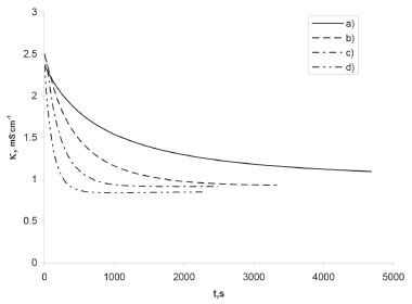
Figure 1. The influence of ester concentration on the evolution of the progression curve of hydrolysis reaction, C_{0, OH-} = 0.01 mol/L; C_{0, AcEth}: a) 0.01, b) 0.02, c) 0.04, d) 0.08 mol/L, respectively

Nonlinear fitting of the data to the equation (5) on the basis of Marquard algorithm was performed using a computer programme that we had developed.

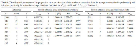
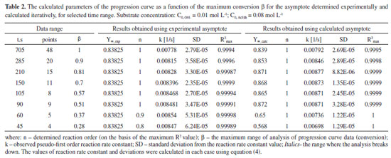
RESULTS AND DISCUSSION

The issue of analysing pseudo-first order reactions

In order to analyse reaction progression curves with the use of the proposed method, we need to be certain that it is indeed described by the first order kinetic equation. In case of homogeneous first order reactions, this is easy to prove. Errors may only arise from selecting the wrong data range for analysis (too low conversion). As for pseudo-first order reactions, additional issues of experimental nature may occur. They revolve around insufficient excess of reagents in relation to the desired one, which would allow us to treat the reaction as a pseudo-first order reaction. This issue is virtually non-existent in the case of acid-catalysed hydrolysis reactions (see: Supplementary Materials), where both acid and water concentrations may be considered constant (very high excess). It is, however, different in the case of alkaline hydrolysis of ester presented below. We need to choose the right reagent concentrations. Obviously, it is also important to select the right data range for the analysis. Both aspects are discussed below.

The effects of the conversion on the results of the progression curve analysis

Given the method used to track the progress of reaction, in this case, it was possible to analyse the impact of the range of the recorded progression curve (conversion) on the value of the calculated rate constant and its statistical parameters. This aspect is not brought up in the literature on progression curves analysis as it is treated as something obvious perhaps. On the other hand, students generally do not realise the significance of the scope of the data analysed. The progression curves of alkaline hydrolysis of an ester (AcEth - ethyl acetate) were selected for the analysis, since they made it possible to record automatically a large amount of data in a wide scope of conversion. This method of recording allows one to choose the conditions of a reaction in such a manner that it is possible to keep track of it until it comes to an end, even in the limited class time. Thus, there is no need to complete the reaction by some other means, e.g. by heating the mixture. This also gives greater confidence that the real, experimental value of the progression curve asymptote will be obtained. Subsequently, the results obtained directly from the real (experimental) data and iteratively determined asymptotes were compared. The detailed analysis is shown below.

For the analysed reaction to be considered a pseudo-first order reaction, a sufficient excess of one of the reacting substances is necessary. ^6,11

Curve a) of Figure 1 shows a second order reaction (equal concentration of the substrates), whereas curve d) already describe a pseudo-first order reaction (sufficient excess of ester in relation to [OH^-]). Case curve b) is relatively complex, since the excess of ester is insufficient for the reaction to be described by a first order equation or a simplified second order equation. Due to the type of reaction presented in this paper, curves c) and d) were analysed and compared. The aim of the comparison is also to possibly detect insufficient substrate (ester) excess in relation to OH^- ions in the case of curve c). As can be seen, in the case of a pseudo-first order reaction, it is important to differentiate between the first order progression curve and the n^th-order progression curve. Suggestions on how to find a solution were provided by Joel Tellinghuisen,¹² the simplest method consisting in comparing the values of R² only. Since in this case the value of Y_∞ may also be needed, it can be determined using the iterative procedure proposed by us. Of course, it is necessary to choose an relevant progression curve equation. The results of the comparison between curves c) and d) progression curve parameters for selected conversion ranges are shown in Tables 1 and 2.

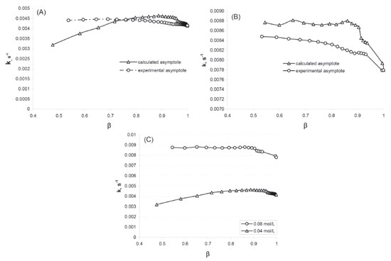
The experimental asymptote is determined from the maximum number of points that was necessary to obtain the constant value of  Y (i.e. Y_∞). This value is then used to check the order and calculate the rate constant for a variable range of the conversion (i.e. a decreasing number of data - a shorter and shorter time interval). As for the calculated asymptote, it is calculated for the systematically shortened range of the progress curve (of data). This is possible until a certain point, but the obtained values differ more and more from the real (experimental) values.

In Table 1, in the case of C_{0, AcEth} = 0.04 mol/L, we can see that below the conversion β = 0.71, the calculated asymptote value begins to differ significantly from the value determined experimentally. It is similar for the observed reaction rate constant, which is additionally illustrated by Figure 2A. The cause is insufficient ester excess in relation to the base which, nevertheless, grows as the reaction progresses. Therefore, in the range of higher conversion, both the reaction order and the rate constant become accurate. The higher number of points (thus their weight) is also significant in the range of higher conversion. By comparing the values presented in Tables 1 and 2, it is relatively easy to see whether the reagent excess is sufficient. If the experimental asymptote is used for calculations, as we limit the range of analysed data towards lower conversion, the observed value of reaction order decreases. Whereas in the case of the iteratively determined asymptote, we can observe a radical change in its value - all the way to meaningless values (even negative value-at t = 180 s). The fact that order 1 shown in the table 1 remains unchanged is only due to the use of the calculated asymptote in that model.

Figure 2. The calculated value of the 1^st Ord. rate constant as a function of the maximum conversion β for the asymptote determined experimentally and calculated iteratively: A) C_{0, OH-} = 0.01 mol/L; C_{0, AcEth} = 0.04 mol/L; B) C_{0, OH-} = 0.01 mol/L; C_{0, AcEth} = 0.08 mol/L. Figure C) shows calculated values of the observed 1st Ord. rate constants as a function of the maximum conversion β for the initial ester concentrations of 0.04 mol L^-1 and 0.08 mol L^-1 respectively. Asymptotes were calculated iteratively

In the case of C_{0, AcEth} = 0.08 mol/L (Table 2), we only observe such unfavourable changes when β is below 0.4. With the growing conversion, the ratio of ester concentration to base concentration increases favourably and thus the values of the calculated parameters become stabilised (Table 2 and Figure 2B). The ratio of the observed reaction rate constants reaches approximately 2 (Figure 2C), so it corresponds to the proportion of ester concentration in both cases (0.08/0.04 = 2). This ratio is a result of the kinetic equation used for the case in question.

By analysing data presented in Tables 1 and 2, we can resolve the issue of sufficient component excess (necessary to facilitate the adoption of the pseudo-first order reaction model) as well as the issue of selecting the data range for analysis. Even sufficient excess does not guarantee the correct calculation of reaction rate constant if there is not sufficient data available on the range of excessively low conversion.

The relationships show us that the fact of better statistical indicators obtained by iterative determination of the value of progression curve asymptote should not be overestimated. This follows from the method itself whereby this value will be fitted to the currently analysed data, even at the expense of departing from the actual value.

From the above-shown relationships, it also follows that the correct calculation of the reaction rate constant with satisfactory statistical characteristics requires an analysis of the progression curve data obtained under the conditions of sufficient excess of ester (chosen substrate). However, the excess does not need to be significant from the very start of the reaction because as the reaction progresses the ratio of the ester concentration to the OH^- ion concentration increases, which defines the pseudo-first order reaction (see Supplementary Material). In such a case, it is sufficient to select data for calculations which include a wide conversion range, as described above. The values obtained on the basis of the experimental and the calculated asymptotes are then consistent with one another. Of course, the data recorded after the reaction has completed should not be used, since this leads to deterioration of the statistical characteristics (see: Table 2, the value β > 0.9). This is probably the effect of decreasing role of variation resulting from the progress of reaction in relation to random variation (measurement errors). Therefore, the optimum conversion range for the progression curve analysis is 0.7-0.9.

CONCLUSIONS

The results obtained confirm the usefulness of the proposed iterative method. Its accuracy is just as good as that of the nonlinear matching method. Due to the simplicity of this solution and the fact that students can implement it unassisted, the proposed approach has, in our opinion, great educational value. It teaches how to optimise the parameters of an experiment, asses the progression curve and apply a simple numerical method in the form of iteration.

As we have observed, the experimental procedures described in laboratory class textbooks entail the risk of major errors. Sources of these errors, even if they can be predicted, may be hard to eliminate. For instance, as a result of heating a mixture in order to complete a reaction, its composition may change due to partial evaporation of components. Careless heating of a mixture of sugars may in turn cause them to undergo caramelisation.

The proposed method makes it possible to avoid determining experimentally the limit value of the measured parameter, which also means that time is saved that otherwise would be needed to determine it.

It is to be noted, however, that regardless of the selected way of determining the asymptote, the progression curve range should include sufficient conversion range, preferably between 0.7 and 0.9. Sometimes this may be difficult to achieve in the average laboratory class time of 2.5 hours during which, when using classical analysis methods (titration, non-automatic reading the angle of rotation of polarized light), it is possible to analyse a reaction in the range of lower conversion. The condition is sufficient initial substrate excess. The excess may also be a result of the nature of the reaction (i.e. one of the substrates being a solvent). For the pseudo-first order reactions accounted for in this paper, the possible use of automatic recording (as in the third experiment: see Supplementary Material) should allow such a selection of parameters (e.g. concentrations of substrates, catalyst, temperature) in order for the reaction to be faster and reach earlier sufficient conversions without significantly reducing the number of measurements.

SUPPLEMENTARY MATERIAL

Supplementary Material include:

• The algorithm (flowchart) of iterative selection of limit value of Y_∞ of the measured parameter.

• Experimental procedures and results of the three student experiments.

• Implementation of the algorithm in Excel spreadsheet.

REFERENCES

1. Bain, K.; Towns, M. H.; Chem. Educ. Res. Pract. 2016, 17, 246.

2. Burewicz, A.; Miranowicz, N.; Chem. Educ. Res. Pract. 2006, 7, 1.

3. Holt, M. J. J.; Norris, A. C.; J. Chem. Educ. 1977, 54, 426.

4. Atkins, P.; De Paula, J.; Atkins' physical chemistry, 8^th ed., W. H. Freeman and Company: New York, 2006, chap. 22.

5. Glenn, V. L.; J. Chem. Educ. 2000, 77, 532.

6. Corbett, J. F.; J. Chem. Educ. 1972, 49, 663.

7. Denton, P.; J. Chem. Educ. 2000, 77, 1524.

8. Borderie, B.; Lavabre, D.; Levy, G.; Micheau, J. C.; J. Chem. Educ. 1990, 67, 459.

9. Hemalatha, M. R. K.; NoorBatcha, I.; J. Chem. Educ. 1997, 74, 972.

10. Schwartz, L. M.; Anal. Chem. 1981, 53, 206.

11. Scilio, F.; Peterson M. D.; J. Chem. Educ. 1961, 38, 576.

12. Tellinghuisen, J.; J. Chem. Educ. 2005, 82, 1709.