JBCS

INTRODUCTION

Currently, new ways are being found to deal with the issue of chemical waste, and new, challenging solutions are proposed to avoid or minimize the production of these wastes before it is necessary to treat them during the process. These alternatives for reducing the impact of chemical activity on the environment are called Green Chemistry.¹

Chemical laboratory activities, by their nature, pose a potential risk of pollution, with toxic or flammable substances producing ‘toxic waste’ after analysis. However, Green Chemistry, also referred to as Clean Chemistry, plays a crucial role in reducing this risk. It advocates for prevention over treatment or cleaning of chemical process residues, thereby lessening the potential harm.²

Another essential principle is real-time analysis to prevent pollution, which is nothing more than the development of analytical methodologies for monitoring and controlling processes in real-time, thus avoiding the generation of harmful substances.³

In this context, water quality monitoring is important to identify the causes that generate pollution from a water source, in addition to assisting in the implementation of best practices for managing healthy ecosystems.^4,5 Normally, water samples are collected in the field and the analyses are done in the laboratory, however, in addition to being laborious and time-consuming, this procedure is expensive and generates chemical waste. Thus, remote sensing combined with machine learning would be a more viable alternative to adapt the monitoring of water sources to the principles of Green Chemistry, because having a large interval of data acquisition, this monitoring could be done via remote sensing.^6,7

Satellite remote sensing has been growing very fast as a technological tool for environmental monitoring, due to the great diversity of sensors capable of capturing and recording the different physical events of the Earth. Through orbital images, high-resolution data are obtained that enable the analysis of parameters such as water quality, through regression models of satellite data and data from analyses of water quality parameters.⁸ This method involves the measurement of electromagnetic radiation emitted or reflected on the water surface. This data can then be transformed and interpreted into parameters, such as water turbidity, offering a greener approach to water monitoring.^9,10

There are examples in the literature of applications of this new technology in which it was possible to estimate pH, dissolved oxygen, electrical conductivity and chlorophyll-a by the remote sensing technique using machine learning in water sources in different regions, showing that the technique can be applied regardless of the location of the study area.^11,12

In this way, remote sensing thus emerges as a cutting-edge and sustainable alternative for monitoring water from sources. Not only does it offer a viable substitute for conventional chemical analysis, but it also mitigates the generation of chemical waste that would otherwise be discarded into the environment, thus moving towards the principles of green chemistry. Of course, one technique is not a substitute for another, especially in this case of orbital water assessment, but it can be much more cost-effective for identifying prone areas and preventing contamination.¹³

Thus, this study aimed to monitor the water quality of the Uberaba River using more sustainable and non-destructive techniques, through orbital remote sensing, and to develop methods for estimating water quality at reduced costs, using orbital sensors and machine learning.

 

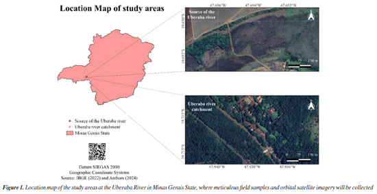
EXPERIMENTAL

Study area description

The values of raw water quality parameters were collected between 2018 and 2023. As shown in the location map (Figure 1), the samples were collected at two locations on the Uberaba River: (i) the source of the river (19°42’48.6”S and 47°56’16.8”W) and (ii) the catchment area of the river (19°39’06.3”S and 47°41’43.9”W).

 

 

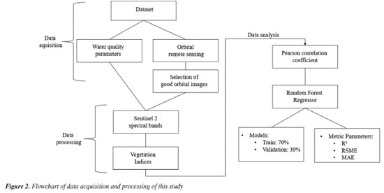
Dataset

The database was composed of water quality parameters provided by CODAU (in Portuguese, this means Companhia Operacional de Desenvolvimento, Saneamento e Ações Urbanas, or Operational Company for Development, Sanitation and Urban Actions) and orbital remote sensing data, obtained free of charge through imaging from the Sentinel-2 constellation, with medium spectral resolution. We chose orbital remote sensing because it is a non-destructive and sustainable method and facilitates access to hard-to-reach areas, as seen in this study, for collecting water quality parameters (Figure 1).

Orbital remote sensing was chosen because the samples were collected in locations with riparian forests, dense vegetation, or difficult access, where aerial imaging or proximal remote sensing would be unfeasible due to the presence of trees, branches, and other obstacles. The vegetation indices were meticulously selected through a thorough brainstorming session, taking into account the indices most commonly used in scientific remote sensing research. This careful selection process ensures the robustness of our research.

The database was meticulously composed, encompassing a range of water quality parameters (chloride, O₂, iron, nitrate, nitrite, ammonia, total phosphorus, total nitrogen, chemical oxygen demand (COD), and biochemical oxygen demand (BOD)). For each parameter, two scenarios were explored using orbital remote sensing. In scenario I, we utilized spectral bands (blue (B), green (G), red (R), red-edge 2 (Re2), near-infrared (NIR), shortwave infrared 1 (SWIR1), and shortwave infrared 2 (SWIR2)) along with a single water quality parameter. In scenario II, we considered vegetation indices such as simple ratio (SR); normalized difference vegetation index (NDVI); normalized difference red edge index (NDRE); nonlinear vegetation index (NLI); normalized difference water index (NDWI); difference vegetation index (DVI); blue-normalized difference vegetation index (BNDVI); inverse of the simple ratio (ISR); green normalized difference vegetation index (GNDVI); red green blue vegetation index (RGBVI); soil adjusted vegetation index (SAVI); chlorophyll index-red edge (CIRE); infrared percentage vegetation index (IPVI); enhanced vegetation index (EVI); and enhanced vegetation index 2 (EVI2) alongside a single water quality parameter. This comprehensive approach ensured that the inputs were spectral bands (scenery I) or vegetation indices (scenery II), and as a response variable of the model, only one water parameter was evaluated at a time, obtaining a model for each parameter, which were carefully considered and evaluated according to the accuracy of each model.

In addition, the dataset was composed of these data and evaluated in function of two scenarios (water parameters and spectral bands; and water parameters and vegetation indices) to investigate the best correlation among the data because we know there are different factors influencing the quality of water and affects the interaction of electromagnetic radiation with water, for example, phytoplankton, organic matter, inorganic minerals and others.^14-16

Data acquisition and processing

Figure 2 demonstrates the robust database, which includes water quality parameters and orbital images sourced from the highly reliable Sentinel‑2 satellite (a passive sensor) of the Copernicus Open Access Hub website.¹⁷ The images were carefully selected, ensuring that only those without clouds or cloud shadows (referred to as ‘good images’) were chosen using the QGIS software, version 3.28.¹⁸ The orbital sensing data (spectral bands and vegetation indices) were extracted from the same location as the collection points’ geographic coordinates, further enhancing the data’s reliability. The wavelengths of the spectral bands used in the research are detailed in Table 1S (Supplementary Material). The vegetation indices were calculated from these wavelengths, as determined by the equations in Table 2S (Supplementary Material).

 

 

Subsequently, the data were analyzed thoroughly and systematically using Pearson’s correlation coefficient to filter data. This approach allowed us to comprehensively understand the dataset and identify the spectral bands and vegetation indices that most strongly correlated with water quality parameters. This thorough analysis instills confidence in selecting the best variables for estimating water quality parameters. Following this, we employed the random forest regressor algorithm to select the best results for water quality parameters.

The data was standardized and GridSearch, a part of the Google Colab library,¹⁹ was used to select the best hyperparameters to estimate each water parameter evaluated. Following this, a random forest regression (RFR) analysis was performed, leveraging the power of a machine learning algorithm. Google Colaboratory,¹⁹ also known as Google Colab, is a platform renowned for its computational capabilities. The data was processed using Python code from the Google Colab website.¹⁹ The dataset was divided into two subsets, 70% for training and 30% for validation, and all the data from this study was validated. The RFR algorithm performed the performance analysis for the spectral bands and vegetation indices. A comprehensive set of metric parameters, including precision (adjusted coefficient of determination, R²) and accuracy (root mean square error (RSME) and mean absolute error (MAE)), were used to evaluate the model validation for each water quality parameter. These metrics provided a robust assessment of the model’s performance, ensuring the reliability of our findings.

Moreover, we chose the random forest algorithm because the data does not present linear behavior. We chose to use the random forest machine learning algorithm, which is widely used to analyze nonparametric data. Furthermore, even if the data has a multicollinearity effect, this does not negatively affect the accuracy and performance of the model, as we can observe in the present work.

 

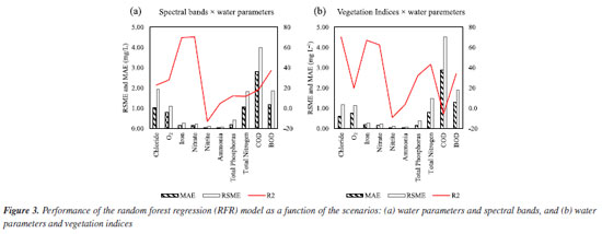
RESULTS AND DISCUSSIONS

Selection of variables for estimation of water parameters

Initially, the remote sensing variables (spectral bands and vegetation indices) most relevant for estimating each water parameter were selected to determine their relationship. For this, Pearson’s correlation coefficient was calculated for each scenario to verify which vegetation bands or indices correlate most with each parameter, as seen in Figures 1S and 2S (Supplementary Material).

For chloride, it is important to note that NIR and Re2 are the ones with the highest correlation coefficient among other spectral bands in scenario I (Figure 1Sa), but it is a weak correlation (less than 0.3). This is a key point, as it suggests that these wavelengths, despite their higher correlation when compared to other wavelengths, may not be the most effective for detecting chloride levels. Similarly, in scenario II (Figure 2Sa), DVI and EVI show a higher correlation coefficient than the others, but also have a weak correlation (less than 0.3), indicating that these wavelengths may not be ideal for this purpose either. This fact was already expected, since the remote sensing of aquatic bodies cannot detect changes in the reflectance of substances that have a lot of interaction with organic matter, since, for example, the reflectance of chlorine changes rapidly by adsorption in organic matter, as chlorine reacts with organic matter and forms other compounds, such as the byproducts of disinfection (trihalomethanes, chlorates, bromates, among others) and this confuses the sensors.²⁰

For dissolved oxygen, in scenario I (Figure 1Sb), it is possible to notice that NIR and Re2 presented a higher correlation coefficient than other wavelengths but also a weak correlation (less than –0.3). In scenario II (Figure 2Sb), DVI and EVI showed a higher correlation coefficient, but the correlation was also weak (less than –0.3). Conversely, for iron in the scenario I (Figure 1Sc), SWIR 1 revealed a moderate negative correlation, with the correlation coefficient ranging between –0.5 and –0.6.²¹ This implies that as the wavelength of the spectral band increases, the iron content decreases, a significant finding for environmental monitoring. In scenario II (Figure 2Sc), the correlation coefficient was higher for NDRE, but since the correlation coefficient is between 0.3 and 0.4, it is a weak correlation.²¹

For nitrate in scenario I (Figure 1Sd), blue presented a higher correlation coefficient than the other spectral bands, but the correlation is weak (less than 0.3). In scenario II (Figure 2Sd), BNDVI presented a higher correlation coefficient, but the correlation was weak (less than –0.3). For nitrite in scenario I (Figure 1Se), the correlation coefficients were very low, with Re2 having the highest correlation coefficient but less than 0.2, which is considered a weak correlation.²¹ In scenario II (Figure 2Se), the correlation coefficients were also lower than 0.2, with the highest being the BNDVI, and therefore the correlation is weak.

For ammonia in scenario I (Figure 1Sf), red showed a higher correlation coefficient than the other spectral bands, but the correlation was weak (less than –0.2). In scenario II (Figure 2Sf), BNDVI had a higher correlation coefficient, but the correlation was weak (less than 0.2). For total phosphorus, NIR displayed a higher correlation coefficient in scenario I (Figure 1Sg), but the correlation was weak (less than 0.2). In scenario II (Figure 2Sg), EVI showed a higher correlation coefficient, but the correlation was also weak (less than 0.3).

For total nitrogen in scenario I (Figure 1Sh), SWIR 1 showed a higher correlation coefficient, but the correlation was weak (–0.3). For scenario II (Figure 2Sh), CIRE showed a higher correlation coefficient, but the correlation was weak (less than 0.4). For COD in scenario I (Figure 1Si), red had a higher correlation coefficient, but the correlation was weak (less than –0.2). In scenario II (Figure 2Si), RGBVI showed a higher correlation coefficient, but the correlation was weak (less than 0.3). For BOD in scenario I (Figure 1Sj), NIR and Re2 showed a higher correlation coefficient, but the correlation was weak (less than 0.2). In scenario II (Figure 2Sj), DVI, SAVI, and EVI2 had a higher correlation coefficient, and the correlation was weak (less than 0.3).

Random forest regression

Figures 3a and 3b show the MAE, RSME and R² of the data for each parameter. The higher the R² value and the lower the values for MAE and RSME, the greater the estimate’s accuracy.²² It can be seen in Figure 3a that for iron and nitrate, the R² value is high. At the same time, MAE and RSME are low, so it is possible to develop a model correlating iron and nitrate with the spectral bands using the RFR algorithm. On the other hand, R² of nitrite, for example, was very low, as was for ammonia and total phosphorus. For COD, total nitrogen, dissolved oxygen, chloride, and BOD, the values of MAE and RSME are very high, which makes it unfeasible to estimate these parameters using RFR using spectral bands.

 

 

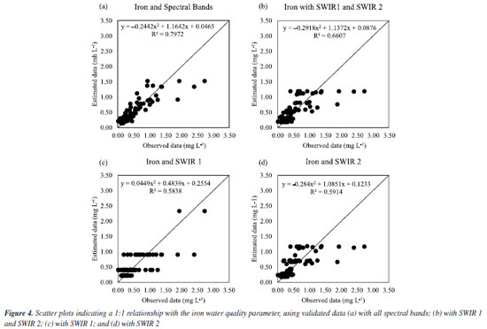
Figure 3b shows that chloride, iron, and nitrate had high R² and low MAE and RSME, which shows that it is possible to estimate these parameters by RFR using vegetation indices. On the other hand, nitrite showed very low R², as well as dissolved oxygen, ammonia, and COD. Therefore, the RFR algorithm is not recommended to estimate these parameters using vegetation indices. BOD, total nitrogen, and COD showed very high MAE and RSME, which shows that estimating these parameters using vegetation indices based on RFR is impossible.

In addition, the dataset was composed of these data and evaluated in function of two scenarios (water parameters and spectral bands; and water parameters and vegetation indices) to investigate the best correlation among the data because we know there are different factors influencing the quality of water and affects the interaction of electromagnetic radiation with water, for example, phytoplankton, organic matter, inorganic minerals and others.^14-16

Performance of validated models

The results, as depicted in Figure 3, underscore the significant performance of the RFR algorithm. It demonstrated unparalleled precision and accuracy in estimating key water quality parameters such as iron, nitrate, chloride, total phosphorus and total nitrogen.

Visual representations of the iron correlation with the spectral bands (scenario I) are presented in Figures 3Sa-3Sd (Supplementary Material). The models, adjustment curves, and coefficient of determination for each situation can be observed in Figures 4a-4d.

 

 

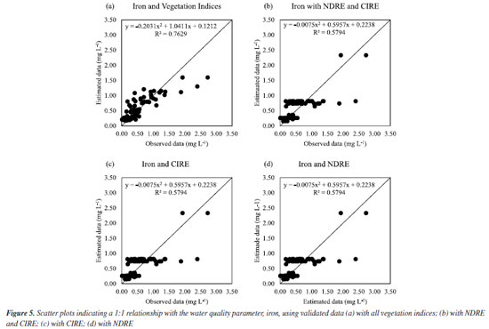
We can see in Figure 3Sa, in which the data were estimated with all spectral bands, the estimated data followed the observed data well, and this fact can be confirmed by Figure 4a, in which it is observed that the data fit well the model and the R² found 79.72%. On the other hand, in Figure 3Sb, estimated only with SWIR 1 and SWIR 2, the estimated data also followed the observed data, but not as precisely as with all spectral bands, as can be seen in Figure 4b, in which it is noted that the data fit less to the model and the R² was 66.07%. By estimating only with SWIR 1 (Figure 3Sc) or only with SWIR 2 (Figure 3Sd), it is observed that the estimated data need to follow the observed data better. From Figures 4c and 4d, it is observed that the R² values obtained were not so impactful, being R² 58.38 and 59.14%, respectively.

Given the above, as shown in Figures 3S and 4, the spectral behavior of water can be affected by the presence of suspended particles (inorganic and organic), dissolved organic substances, and living organisms.²³ The presence of organic matter or organic substances, such as iron and chlorine, observed in this study causes a decrease in reflectance in the visible region, as these elements are absorbed by water.¹⁵ On the other hand, there is a predominance of reflectance in the near-infrared region (Figure 4), as evidenced in this study in the shortwave bands (SWIR 1 and SWIR 2). We estimated these parameters using the random forest algorithm, which resulted in great results with medium (66.07, 58.38, and 59.14%) and high (79.72%) R² values. In addition, the increase in living organisms, such as phytoplankton, results in absorption in the visible region, mainly in the blue and red bands, and in the reflectance of green, near-infrared (NIR), and shortwave (SWIR).

In scenario II, Figure 4Sa correlates with all vegetation indices. It shows that the estimated data followed the observed data better than in Figure 4Sb with only NDRE and CIRE, Figure 4Sc with only CIRE, and Figure 4Sd with only NDRE. Figures 5a-5d confirm the best fit for all vegetation indices since R² was 76.29%. The other results obtained, in Figures 5b-5d, were not so impactful.

 

 

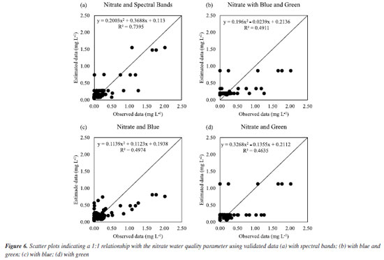
Thus, the best fit for iron is in scenario I. It was already expected that iron could be estimated via orbital remote sensing since iron can give characteristic color to the water since dissolved iron (ferrous ion) transforms into ferric ion (ferric oxide and ferric hydroxide) in contact with air and thus forms rust and this color can be captured in orbital images, once the orbital satellite generates a signal that interacts with water, which generates a signal in the form of spectral bands.^24,25

For nitrate, in scenario I, Figure 5Sa (Supplementary Material), for all spectral bands, it is noted that the estimated data followed the observed data better, and Figure 5Sb, for blue and green, Figure 5Sc for blue only, and Figure 5Sd for green only, the estimated data did not follow the observed data so well. This can be proven by Figure 6a, in which a good fit was obtained, and the R² value was 73.95% with all spectral bands. For Figures 6b-6d we did not obtain such an impactful R².

 

 

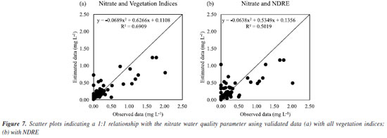
For nitrate, in scenario II, it can be seen from Figure 6Sa (Supplementary Material), with all vegetation indices, that the estimated data followed the observed data better than with NDRE alone, Figure 6Sb. This fact is confirmed by Figure 7a, in which a good fit was obtained, and R² was 69.09%, while in Figure 7b, we can see that R² was not so impactful.

 

 

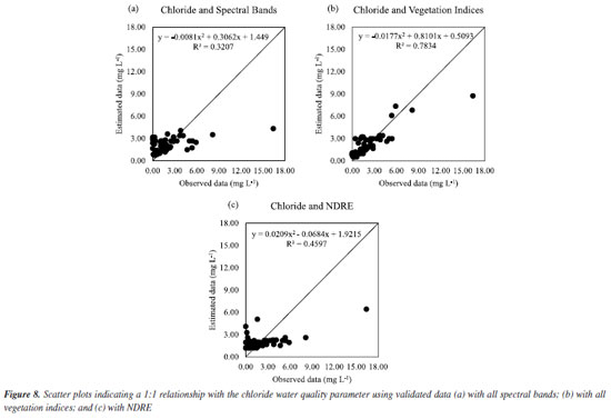
Thus, in the case of nitrate, the best way to estimate it would be with all spectral bands (scenario I). Another study²⁶ also sought to estimate nitrate using a model obtained by the RFR for groundwater and found an adjustment with R² of 89.10%.

For chloride, in scenario I, Figure 7Sb (Supplementary Material) shows that the estimated data followed better the data observed with all vegetation indices (scenario II) than with all spectral bands (Figure 7Sa) and only with NDRE (Figure 7Sc). This can be confirmed by Figure 8b, in which a good fit was obtained with R² of 78.34%. For Figures 8a and 8c, R² was not impactful.

 

 

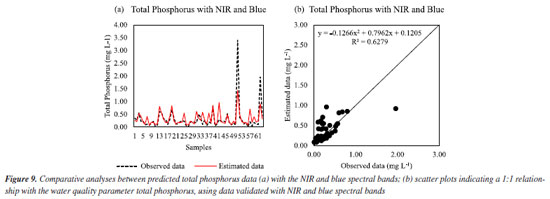
Thus, the best fit to estimate chloride by the RFR was scenario II, with all vegetation indices. Another study²⁷ was also able to obtain a regression model for chloride using Sentinel 2A images and obtained an R² of 80.80%.

For total phosphorus, the best regression was for scenario I with only NIR and blue, as seen in Figure 9a. The estimated data followed the observed data well, with R² of 62.79%. This is considered a low value, since phosphorus is important in the detection of eutrophication of surface water sources.²⁸ A recent study²⁹ also sought to obtain a regression with an algorithm correlating the reflectance of remote sensing with the values of parameters contained in surface waters. An adjustment with R² of 75.96% was found for the total phosphorus.

 

 

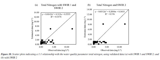
For total nitrogen, the estimated data better matched the data observed with SWIR 1 and SWIR 2, as seen in Figure 8Sa (Supplementary Material) and confirmed in Figure 10a, in which an adjustment with R² of 55.76% was obtained. It should be noted that using RFR did not obtain an impactful R² value. A survey also used Sentinel-2 images to obtain a regression model to estimate nitrogen using orbital remote sensing obtained in two distinct regions: in one region it was obtained an R² of 67.00%, and in another region, an R² of 78.32%.³⁰

 

 

For COD, it is observed that the estimated data did not follow the observed data well, as can be seen in Figures 9Sa and 9Sb (Supplementary Material). This can be confirmed by Figures 11a and 11b, in which R² could have been more impactful. Thus, for COD, the RFR models are not the most appropriate to estimate this parameter, and it is necessary to test other regression algorithms.

 

 

Thus, it is possible to estimate iron, nitrate, chloride, total phosphorus, and total nitrogen using Sentinel-2 orbital images and machine learning using the RFR algorithm. This more sustainable technique could avoid generating waste from conventional chemical analyses. In summary, Table 3S (Supplementary Material) shows the best validation models to estimate iron, nitrate, chloride, total phosphorus, and total nitrogen.

Economic analysis

The orbital remote sensing part did not generate any cost to carry out this work. The costs of conventional chemical analysis can be seen in Table 4S (Supplementary Material). In addition to these costs, there is the cost of traveling to collect samples. Thus, this new method of analysis, besides being sustainable, represents a saving of 100% compared to conventional analyses.

 

CONCLUSIONS

It can be concluded that it is possible to perform orbital remote sensing by performing the regression by the random forest regression correlating the information obtained from Sentinel-2 images and the values of iron, nitrate, chloride, total phosphorus, and total nitrogen parameters, being a sustainable technique, which does not generate any waste, in addition to representing a 100% saving in relation to conventional chemical analyses. This approach can be very helpful to monitor and prevent contamination, but of course does not replace the chemical analyses for certain variables. On the other hand, can be much more effective to map and find the cause of contamination.

 

SUPPLEMENTARY MATERIAL

Tables referring to spectral bands, vegetation indices, validation models to estimate the water parameters and costs of conventional chemical analyses (Tables 1S-4S), as well as figures referring to Pearson’s correlation coefficient analyses (Figures 1S-2S) and comparative analyses (Figures 3S-9S) are freely available at http://quimicanova.sbq.org.br, in PDF format.

 

ACKNOWLEDGMENTS

The authors thank the funding agencies CAPES, CNPq (313447/2021-7) and FAPEMIG (PPM 00147-17). The authors also thank the Companhia Operacional de Desenvolvimento, Saneamento e Ações Urbanas (CODAU) for providing the data used in this study.

 

REFERENCES

1. Lenardão, E. J.; Freitag, R. A.; Dabdoub, M. J.; Batista, A. C. F.; Silveira, C. C.; Quim. Nova 2003, 26, 123. [Crossref]

2. da Silva, F. M.; de Lacerda, P. S. B.; Jones Junior, J.; Quim. Nova 2005, 28, 103. [Crossref]

3. Strinta, L. P. T.: A Política de Economia Circular da União Europeia e sua Integração com os Princípios da Química Verde: Uma Pesquisa Documental; Final Paper, Universidade Federal de São Carlos, Araras, São Paulo, Brazil, 2024. [Link] accessed in October 2024

4. Naimaee, R.; Kiani, A.; Jarahizadeh, S.; Asadollah, S. B. H. S.; Melgarejo, P.; Jodar-Abellan, A.; Sustainability 2024, 16, 646. [Crossref]

5. Aqel, H.; Sannan, N.; Al-Hunaiti, A.; Fodah, R.; PLoS One 2024, 19, e0298200. [Crossref]

6. Leggesse, E. S.; Zimale, F. A.; Sultan, D.; Enku, T.; Srinivasan, R.; Tilahun, S. A.; Hydrology 2023, 10, 110. [Crossref]

7. Gao, L.; Shangguan, Y.; Sun, Z.; Shen, Q.; Shi, Z.; Remote Sens. 2024, 16, 514. [Crossref]

8. Giménez, J. G.; González, M.; Martínez-España, R.; Cecilia, J. M.; López-Espín, J. J.; Journal of Ambient Intelligence and Smart Environments [Crossref]

9. Carneiro, F. M.: Sensores de Dossel no Monitoramento da Variabilidade Temporal das Culturas da Soja e do Amendoim; PhD Thesis, Universidade Estadual Paulista Júlio de Mesquita Filho, Jaboticabal, São Paulo, Brazil, 2018. [Link] accessed in October 2024

10. de Brito, H. C.; Vasconcelos, R. S.; Rufino, I. A. A.; de Brito, Y. M. A.; Caminhos de Geografia 2022, 23, 108. [Crossref]

11. Lamrini, M.; Mahria, B. B.; Chkouri, M. Y.; Touhafi, A.; Sensors 2024, 24, 4084. [Crossref]

12. Efriana, A. F.; Manessa, M. D. M.; Ayu, F.; Damayanti, A.; Haidar, M.; Setiawan, K. T.; Geosfera Indonesia 2024, 9, 144. [Crossref]

13. Sagan, V.; Peterson, K. T.; Maimaitijiang, M.; Sidike, P.; Sloan, J.; Greeling, B. A.; Maalouf, S.; Adams, C.; Earth-Sci. Rev. 2020, 205, 103187. [Crossref]

14. Cabral, A. P.; Mantovani, J. E.; Costa, M. P. F.; de Lima, R. F.; Novo, E. M. M. L.; Simpósio Brasileiro de Sensoriamento Remoto; São José dos Campos, Brazil, 1990. [Link] accessed in October 2024

15. Mantovani, J. E.: Comportamento Espectral da Água: Faixas Espectrais de Maior Sensibilidade ao Fitoplâncton na Presença de Matéria Orgânica Dissolvida e de Matéria Inorgânica Particulada; Master’s Thesis, Instituto Nacional de Pesquisas Espaciais, São José dos Campos, Brazil, 1993. [Link] accessed in October 2024

16. Moreira, M. A.; Fundamentos do Sensoriamento Remoto e Metodologias de Aplicação, 4^th ed.; UFV: Viçosa, 2012.

17. Copernicus Browser, https://browser.dataspace.copernicus.eu/, accessed in October 2024.

18. Sherman, G.; QGIS Software, v.3.28; Open Source Geospatial Foundation Project, Italy, 2002.

19. Google Colab, https://colab.google/, accessed in October 2024.

20. Meyer, S. T.; Cadernos de Saude Pública 1994, 10, 99. [Crossref]

21. Costa, M. F. B.; dos Santos, J. A. N.; International Journal of Energy Economics and Policy 2020, 10, 102. [Crossref]

22. Koh, J. C. O.; Hayden, M.; Daetwyler, H.; Kant, S.; Plant Methods 2019, 15, 64. [Crossref]

23. Novo, E. M. L. M.; Sensoriamento Remoto: Princípios e Aplicações, 4^th ed.; Blucher: São Paulo, 2010.

24. de Carvalho, A. R.; Anais do XIII Congresso Brasileiro de ÁguasSubterrâneas; São Paulo, Brazil, 2004. [Link] accessed in October 2024

25. Clark, P. E.; Rilee, M. L.; Remote Sensing Tools for Exploration; Springer: New York, 2010, p. 1. [Crossref]

26. Cardenas-Martinez, A.; Rodriguez-Galiano, V.; Luque-Espinar, J. A.; Mendes, M. P.; J. Hydrol. (Amsterdam, Neth.) 2021, 603, 127092. [Crossref]

27. Mohandas, K. A.; Brema, J.; J. Sci. Ind. Res. 2023, 82, 466. [Crossref]

28. Braga, E. A. S.: Determinação dos Compostos Inorgânicos Nitrogenados (Amônia, Nitrito e Nitrato) e Fósforo Total, na Água do Açude Gavião, e sua Contribuição para a Eutrofização; Master’s Thesis, Universidade Federal do Ceará, Fortaleza, Ceará, Brazil, 2006. [Link] accessed in October 2024

29. Lu, S.; Deng, R.; Liang, Y.; Xiong, L.; Ai, X.; Qin, Y.; Remote Sens. 2020, 12, 1420. [Crossref]

30. Li, J.; Wang, J.; Wu, Y.; Cui, Y.; Yan, S.; Frontiers in Environmental Science 2022, 10, 1014155. [Crossref]

 

Associate Editor handled this article: Cassiana C. Montagner